The steps below are summarized (and simplified) notes from the paper (McInnes, Healy, and Melville 2018) and the ideas from the great medium article (Oskolkov 2019).

Algorithm 

Constructing the High Dimensional Graph Representation (top_rep) 

top_rep is a weighted k-nearest neighbor graph of the high dimensional data.

Let \(X = \{\vec{x}^{(1)}, \vec{x}^{(2)}, …, \vec{x}^{(N)}\}\), \(\vec{x}^{(i)} \in ℝ^{D}\) be the input dataset, with a metric (hyperparameter) \(d : X × X → ℝ_{≥ 0}\)

top_rep is represented as a graph: G = (V, E, w).

The vertices V of G are the data points X.

Given an input hyperparameter k, the edges are the set :

$$ E = \{(\vec{x}^{(i)}, \vec{x}^{(i_{j})}) \ | \ 1 \leq j \leq k, 1 \leq i \leq N\} $$

UMAP uses nearest neighbor descent to compute the k nearest neighbors \(\{\vec{x}^{(i_{1})}, \vec{x}^{(i_{2})}, …,\vec{x}^{(i_{k})}\}\) of a point \(\vec{x}^{(i)}\) given a distance metric d().

The weights of the high dimensional graph are defined by:

$$ w_{i, j}^{i} = w((\vec{x}^{(i)}, \vec{x}^{(i_{j})})) = \exp\bigg(\dfrac{-\max(0, d(\vec{x}^{(i)}, \vec{x}^{(i_{j})}) - \rho_{i})}{\sigma_{i}}\bigg) $$

where \(w_{i, j}^{i}\) is the weight between points \(\vec{x}^{(i)}\) and \(\vec{x}^{(j)}\) w.r.t \(\vec{x}^{(i)}\) and \(\rho_{i}\) is the distance from each i-th data point to it’s first nearest neighbor.

$$ \rho_{i} = \min\{d(\vec{x}^{(i)}, \vec{x}^{(i_{j})}) \ | \ 1 \leq\ j \leq k, d(\vec{x}^{(i)}, \vec{x}^{(i_{j})}) \geq 0 \} $$

\(σ_{i}\) is found through binary search and is defined (based on empirical experiments) such that:

$$ \sum_{j=1}^{k}\exp\bigg(\dfrac{-\max(0, d(\vec{x}^{(i)}, \vec{x}^{(i_{j})}) - \rho_{i})}{\sigma_{i}}\bigg) = \log_{2}(k) $$

Notice that the max value of \(w((\vec{x}^{(i)}, \vec{x}^{(i_{j})}))\) is 1 for close points, and  → 0 for faraway neighbors.

The component \(\dfrac{- \max(0, d(\vec{x}^{(i)}, \vec{x}^{(i_{j})}) - \rho_{i})}{\sigma_{i}}\)

accounts for the locally varying distance metric, because it makes the weight computation unique for each data point.

The local connectivity constraint is also obeyed because each point x_i is connected to atleast one other point with a weight \(w = 1\).

Because the distances between points are not symmetric and are incompatible (there are two edges between points representing d(a, b) and d(b, a)), they are combined using the fuzzy union.

$$ \overline{w_{i,j}} = w_{i, j} + w_{j, i} - w_{i, j}w_{j, i} $$

Constructing the Low Dimensional Representation 

The low dimensional representation \(Y = \{\vec{y}^{(1)}, \vec{y}^{(2)}, …, \vec{y}^{(N)}\}\), \(\vec{y}^{(i)} \in ℝ^{d}\) and \(d \ll D\) is initialized using spectral embedding.

The resulting initialization is optimized using Stochastic Gradient Descent (SGD) with the cross entropy loss: $$ L = \sum_{e \in E}\bigg(w_{h}(e)\log\bigg(\frac{w_{h}(e)}{w_{l}(e)}\bigg) + (1-w_{h}(e))\log\bigg(\frac{1-w_{h}(e)}{1-w_{l}(e)}\bigg)\bigg) $$

UMAP defines the weights of the low dimensional graph, w_l(e), as:

$$ w_l(e(\vec{y}^{(i)}, \vec{y}^{(j)})) = \bigg( 1 + a(\lVert \vec{y}^{(i)} - \vec{y}^{(j)} \rVert_{2}^{2})^{b}\bigg)^{-1} $$

with \(a,b > 0\) and \(\vec{y}^{(i)}, \vec{y}^{(j)} \in \mathbb{R}^{d}\)

Observe that for faraway points \(w_{l}→ 0\), for close points \(w_{l} → 1\), which is desired.

The values a and b are computed using non-linear least squares fitting:

$$ \bigg( 1 + a(\lVert \vec{y}^{(i)} - \vec{y}^{(j)} \rVert_{2}^{2})^{b}\bigg)^{-1} \approx \begin{cases} 1, & if \ \lVert \vec{y}^{(i)} - \vec{y}^{(j)} \rVert_{2} \leq \min\_dist,\\ \exp\bigg(-\lVert \vec{y}^{(i)} - \vec{y}^{(j)} \rVert_{2} - \min\_dist\bigg) & otherwise \end{cases} $$

This implies that in the embedding space, points that are less than min_dist apart get a weight of 1 in the low dimensional embedding. min_dist accounts for the super tightly packed clusters observed in UMAP.

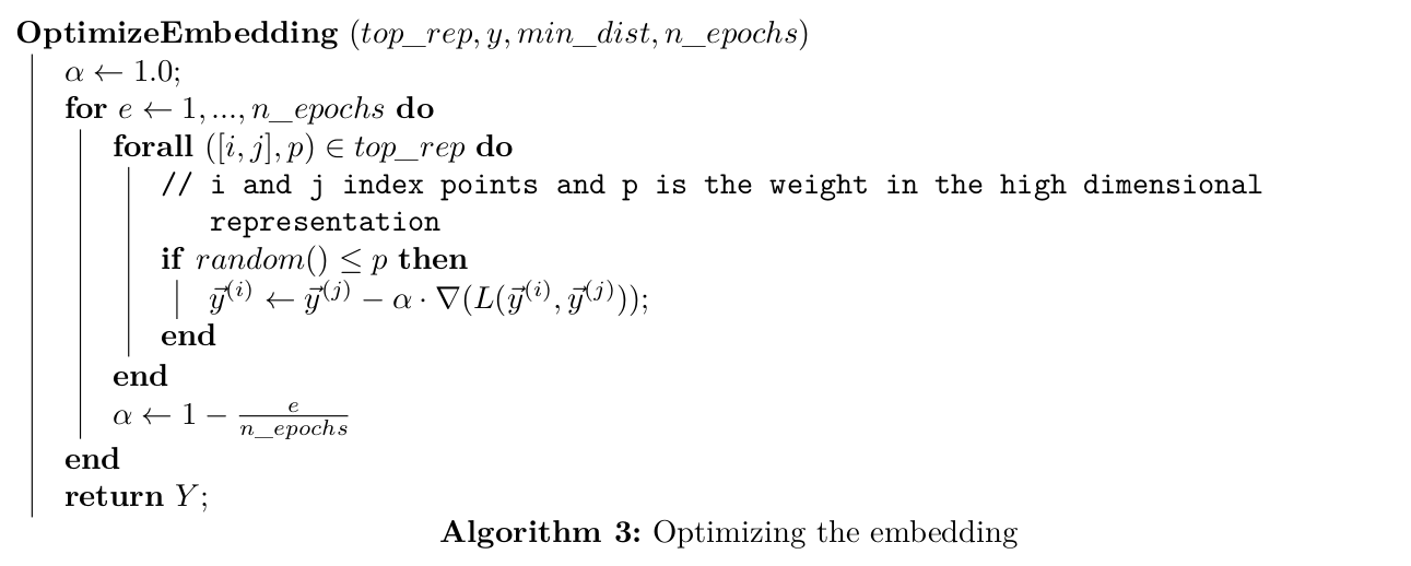
Now that we have the low dimensional initialization and the loss function we can use SGD to optimize this low dimensional representation.

Note: The SGD algorithm above is simplified for understanding, the actual implementation uses additionally negative sampling.

References

Oskolkov, Nikolay. 2019. “How Exactly UMAP Works. And Why Exactly It Is Better Than tSNE | by Nikolay Oskolkov | Towards Data Science.” https://towardsdatascience.com/how-exactly-umap-works-13e3040e1668.